DNA sequence classification via an EM algorithm

Implementation of the SeqEM algorithm

Introduction

In the article , the authors describe a new approach to determine for an individual whether or not a genetic variation is found at a specific position in a genome. The authors propose a new method, based on the EM algorithm, called SeqEM, which is supposed to be more precise and accurate than the methods that have existed until now. The goal is to implement the algorithm by hand in R.

Here, we propose a novel genotype-calling algorithm that, in contrast to the other methods, estimates parameters underlying the posterior probabilities in an adaptive way rather than arbitrarily specifying them a priori. The algorithm, which we call SeqEM, applies the well-known Expectation-Maximization algorithm to an appropriate likelihood for a sample of unrelated individuals with next-generation sequence data, leveraging information from the sample to estimate genotype probabilities and the nucleotide-read error rate.

Context

The element that represents a position in the DNA is called a nucleotide. So to identify the genotype of an individual, the genome of the individual is compared to a reference genome. This is equivalent to comparing the nucleotides of the individual’s genome to the nucleotides of the reference genome. If the nucleotide is identical to the reference nucleotide it is said to be a reference nucleotide (R), otherwise it is said to be a variant nucleotide (V). However, it is not possible to compare the entire DNA to the reference DNA. We therefore choose a fragment of the DNA that interests us (genetic region of interest) and we “copy” (by amplification) this fragment several times. Afterwards, we can align all these fragments with the genetic region of interest of the reference genome. The number of overlaps of these DNA fragments is called reading depth, which we will note N. One is then able to count, line by line, for each nucleotide in this “overlap area” the number of reference and variant nucleotides. The number of variant nucleotides X, which can vary between 0 and N, is noted at a precise position. For a given position in the DNA, i.e. a certain nucleotide, 3 types (genotypes) of individuals can be distinguished:

VV homozygotes \(\rightarrow\) \(N\) variant nucleotides
RR homozygotes \(\rightarrow\) \(N\) reference nucleotides
(RV) heterozygotes \(\rightarrow\) mixture between variant and reference nucleotides

In a perfect world one would therefore, theoretically, be able to identify with certainty the genotype of an individual. However, we are faced with a certain “nucleotide reading error”, which may, for example, be due to errors in the coding of DNA fragments. This error then allows certain nucleotides to be incorrectly encoded and, for example, an RR homozygote presents a nucleotide varying at the position of interest in one of the aligned DNA fragments. Moreover, the number of observed variant nucleotides X does not only depend on the risk of this error, which we will note \(\alpha\), but also on the reading depth N. The probability of observing a variant nucleotide at a given position in the DNA fragment in an RR homozygote is therefore no longer 0, but \(\alpha\). We can see that the larger the \(\alpha\) and the smaller the \(N\), the more difficult it will be to determine the true genotype.

We deduce that, for example if the individual is a RR homozygous, the probability of observing \(X\) variant nucleotides on \(N\) nucleotides in total is \(\binom{N_i}{X_i}. \alpha^{X_i} (1-\alpha)^{N_i-X_i}\), because there are \(\binom{N_i}{X_i}\) possibilities to observe \(X\) variant nucleotides among \(N\) nucleotides and the probability to observe exactly \(X\) variant nucleotides is \(\alpha^{X_i} (1-\alpha)^{N_i-X_i}\). We can then conclude that the number of variant nucleotides observed has a binomial distribution. We find the same results (with obviously other parameter values) for the two other genotypes.

The model

Let \(\mathbf{N_i}\) be the reading depth set for the individual \(i\).

Remark. In the following we will treat the \(N_i\) rather as fixed values and not as parameters. For the simulations we will even note that \[\forall i \in \{1,\dots,S\}, \quad N_i = N\]

We designate by

\(\boxed{X_i \in \{0,\ldots,N_i\}}\) the number of observed variant nucletoides \(i\)
\(\boxed{Z_i \in \{\text{RR, VV, RV}\}}\) the true genotype of the individual \(i\)

We note \(\boxed{\theta = \left(\alpha, p_{\text{VV}}, p_{\text{RV}}\right)}\) , where

\(\alpha\) is the reading error, i.e. the probability that a \(R\) nucleotide is wrongly identified as \(V\) and vice versa.
\(p_{\text{VV}}\) and \(p_{\text{RV}}\) are the proportions of \(VV\) and \(RV\) genotypes in the population \(\Longrightarrow\) \(1-p_{\text{VV}}-p_{\text{RV}}\) is the proportion of \(RR\) genotype in the population

So, we find that

\(\mathbb{P}(Z_i = \text{VV} | \theta) = p_\text{VV}\)
\(X_i | Z_i=\text{VV} \sim B(1-\alpha,N_i)\)

\(\mathbb{P}(Z_i = \text{RV} | \theta) = p_\text{RV}\)
\(X_i | Z_i=\text{RV} \sim B\left(0.5,N_i\right)\)

\(\mathbb{P}(Z_i = \text{RR} | \theta) = 1-p_\text{VV}-p_\text{RV}\)
\(X_i | Z_i=\text{RR} \sim B(\alpha,N_i)\)

Knowing that \(\mathbb{P}\left(X_i, Z_i | \theta \right) = \mathbb{P}(Z_i | \theta) \times \mathbb{P}(X_i | Z_i, \theta)\), we find that

\(\boxed{\mathbb{P}\left(X_i, Z_i=\text{VV} | \theta \right) = \binom{N_i}{X_i} (1-\alpha)^{X_{i}} \alpha^{N_{i}-X_{i}} p_{\text{VV}}}\)
\(\boxed{\mathbb{P}\left(X_i, Z_i=\text{RV} | \theta \right) = \binom{N_i}{X_i}\left(\frac{1}{2}\right)^{N_i} p_{\text{RV}}}\)
\(\boxed{\mathbb{P}\left(X_i, Z_i=\text{RR} | \theta \right) = \binom{N_i}{X_i} \alpha^{X_i} (1-\alpha)^{N_i-X_i} (1-p_{\text{VV}}-p_{\text{RR}})}\)

Knowing that the pairs \(\left(\left(X_{i}, Z_{i}\right)\right)_{1 \leq i \leq n}\) are independent, \[ \boxed{\mathbb{P}(X, Z | \theta)=\prod_{i=1}^{n} \mathbb{P}\left(X_{i}, Z_{i} | \theta\right)} \]

Simulations

In order to better understand the problem and to recognize why an algorithm such as SeqEm is needed to determine the genotype, some simulations will be carried out to understand the motivations behind the development of such an algorithm.

To carry out this simulation we distinguish 4 steps:

A number of individuals \(S\) is chosen, as well as the proportions of VV homogyzotes and heterogyzotes in the population (\(p_\text{VV}\) and \(p_\text{RV}\)).
A sample of size \(S\) of the genotypes (variable \(Z_i\)) of the \(S\) individuals is generated according to a multinomial distribution defined by the parameters \(p_\text{VV}\) and \(p_\text{RV}\).
For the reading depth \(N\) and the reading error \(\alpha\), we simulate for each individual \(i\) according to the law of \(X_i | Z_i\) the number of observed variant nucleotides.
Steps 1 - 3 are repeated for different values of \(N\) and \(\alpha\).

To simplify this procedure, steps 1-3 are integrated into a function called data_generation which, depending on the user’s choice, generates a graphical representation of the \(X_i\) and/or returns the vectors of the \(X_i\) and \(Z_i\).


## Step 1 :
S = 500    # number of individuals
pVV = 0.4  # proportion of VV homozygotes in the population
pRV = 0.3  # proportion of heterozygotes in the population

data_generation = function(S, pVV, pRV, N, alpha, getData=FALSE, plot=FALSE){
	
	## Step 2 : Simulation of a sample of genotypes of all S individuals  
	Z = sample(x = c("VV", "RV", "RR"),
				size = S,
				replace=TRUE,
				prob = c(pVV, pRV, 1-pVV-pRV))
	
	N = rep(N,S)   # vector of reading depths for all individuals
	X = rep(NA,S)  # vector of the number of variant nucleotides variants for all individuals
	
	## Step 3 : Simulation of the number of variant nucleotides for each individual
	#  (according to his genotype)
	for (i in 1:S){
	if (Z[i]=="VV"){X[i]=rbinom(1,N[i],1-alpha)}
	else if (Z[i]=="RV"){X[i]=rbinom(1,N[i],0.5)}
	else {X[i]=rbinom(1,N[i],alpha)}
	}
	
	if (plot==TRUE){
	# One-dimensional scatter plot and histogram
	par(mfrow=c(1,2), mar=c(13,5,5,2), xpd=TRUE)
	plot(1:S, X,
			col=ifelse(Z=="RV","green",ifelse(Z=="VV","blue","red")), xlab="Individuals")
	legend("topleft",
			inset=c(0,-0.45),
			legend=c("VV","RV","RR"),
			col=c("blue","green","red"),
			title="Genotypes",
			pch=1, cex=0.35)
	par(mar=c(13,2,5,2))
	hist(X, breaks=30, main="")
	}
	if(getData==TRUE){return(list(X=X, Z=Z))}
}

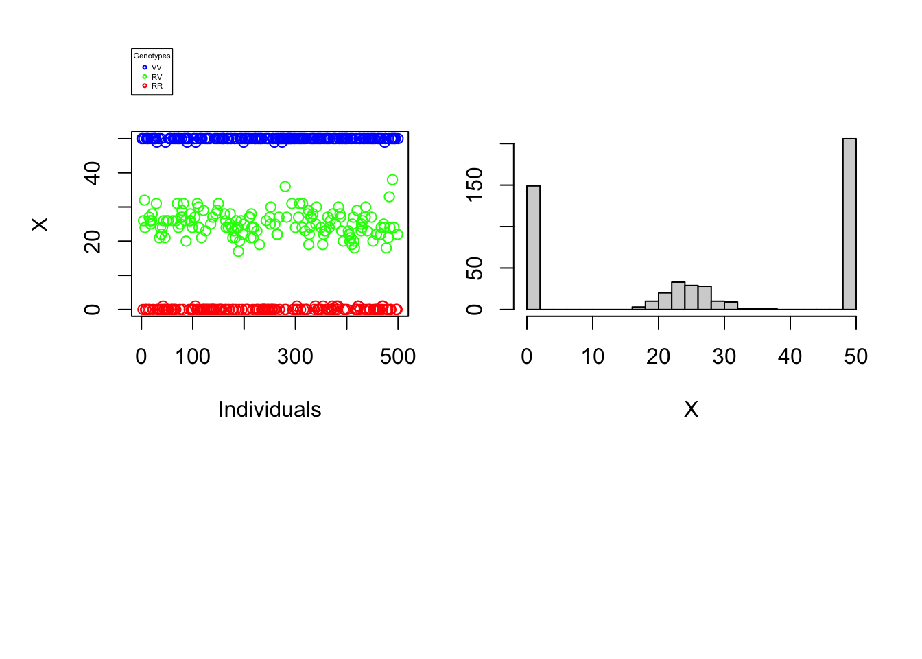
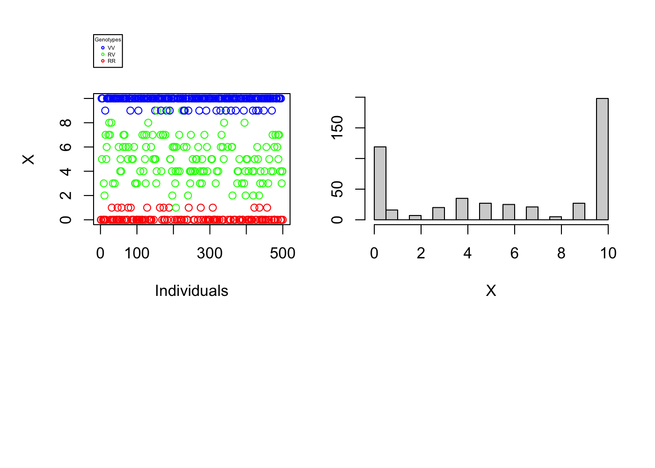
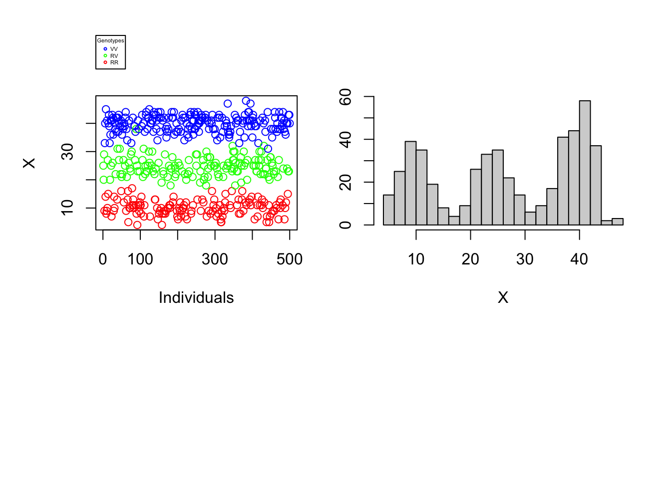
Since the difficulty of determining an individual’s genotype depends neither on the number of individuals nor on the proportions of different genotypes in the population, our understanding of the problem would not be broadened by varying these parameters. The reading error \(\alpha\) as well as the reading depth \(N\) can, on the other hand, make the complexity of genotyping more or less difficult. The graphs below will help to illustrate this finding. For each vector \(X\) a one-dimensional scatterplot and a histogram is generated.


set.seed(1)
## Step 4

data_generation(S, pVV, pRV, N=50, alpha=0.001, plot=TRUE)


data_generation(S, pVV, pRV, N=10, alpha=0.01, plot=TRUE)


data_generation(S, pVV, pRV, N=50, alpha=0.2, plot=TRUE)


ata_generation(S, pVV, pRV, N=10, alpha=0.2, plot=TRUE)

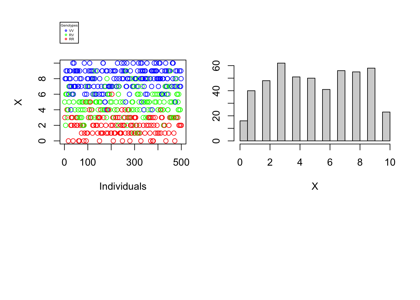
It is immediately noticeable that for \(N\) rather large and \(\alpha\) rather small one can easily distinguish the genotypes of the different individuals using the number of variant nucleotides. \(\rightarrow\) Figure 1. Graphically, lines could even be added to the histogram and scatter plot to separate the 3 genotypes. On the other hand, if the reading depth is small and/or if the reading error is large, one is no longer able to clearly distinguish the different genotypes by observing the number of variant nucleotides..

A posteriori distribution: \(\mathbb{P}(Z | X ; \theta)\)

\[\begin{align*} \mathbb{P}\left(Z_{i}=k | X_{i} , \theta \right) &=\frac{\mathbb{P}\left(X_{i} | Z_{i}=k, \theta\right) \mathbb{P}\left(Z_{i}=k | \theta \right)}{\mathbb{P}\left(X_{i} |\theta \right)} \\ & = \frac{\mathbb{P}\left(X_{i} | Z_{i}=k, \theta\right) \mathbb{P}\left(Z_{i}=k | \theta \right)}{\mathbb{P}\left(X_{i} | Z_{i}=\text{VV} , \theta\right) \mathbb{P}\left(Z_{i}=\text{VV} | \theta\right) + \mathbb{P}\left(X_{i} | Z_{i}=\text{RV}, \theta\right) \mathbb{P}\left(Z_{i}=\text{RV} | \theta \right) + \mathbb{P}\left(X_{i} | Z_{i}=\text{RR}, \theta \right) \mathbb{P}\left(Z_{i}=\text{RR} | \theta \right)} \\ & = \frac{\mathbb{P}\left(X_{i} | Z_{i}=k, \theta \right) \mathbb{P}\left(Z_{i}=k | \theta \right)}{\mathbb{P}\left(X_{i} | Z_{i}=\text{VV}, \theta \right) \times p_\text{VV} + \mathbb{P}\left(X_{i} | Z_{i}=\text{RV}, \theta \right) \times p_\text{RV} + \mathbb{P}\left(X_{i} | Z_{i}=\text{RR}, \theta \right) \times (1-p_\text{VV}-p_\text{RV})} \end{align*}\]

\(Q(\theta | \theta^{\text{old}})\) and its derivatives and formulas for the E/M steps

We know that if the pairs \(((X_i,Z_i))_{1\leq i \leq S}\) are independent, then

\[ Q(\theta | \theta^{\text{old}}) = \sum_{i=1}^{n} \left\{ \int_{Z_{i}} \mathbb{P}\left(Z_{i} | X_{i}, \theta_{\text {old}}\right) \log \left[\mathbb{P}\left(X_{i}, Z_{i} | \theta\right)\right] d Z_{i} \right\} \]

We have

\[\begin{align*} \log \left[\mathbb{P}\left(X_{i}, Z_{i} | \theta\right)\right] = & \left[\log\left(f_{B(1-\alpha,N_i)}(X_i)\right) + \log(p_{\text{VV}})\right] \times \mathbb{1}_{\{Z_i=\text{VV}\}} \\ & + \left[\log\left(f_{B(0.5,N_i)}(X_i)\right) + \log(p_{\text{RV}})\right] \times \mathbb{1}_{\{Z_i=\text{RV}\}} \\ & + \left[\log\left(f_{B(\alpha,N_i)}(X_i)\right) + \log(1-p_{\text{VV}}-p_{\text{VV}})\right] \times \mathbb{1}_{\{Z_i=\text{RR}\}} \end{align*}\]

and

\[\begin{align*} \eta_{\text{VV}}(i) &= \mathbb{P}\left(Z_{i} = \text{VV} | X_{i}, \theta_{\text {old}}\right) \\ &= \frac{\binom{N_i}{X_i} (1-\alpha_{old})^{X_{i}} \alpha_{old}^{N_{i}-X_{i}} p_\text{VV}^{old}}{\binom{N_i}{X_i} (1-\alpha_{old})^{X_{i}} \alpha_{old}^{N_{i}-X_{i}} p_\text{VV}^{old} + \binom{N_i}{X_i} \left(\frac{1}{2}\right)^{N_i} p_\text{RV}^{old} + \binom{N_i}{X_i} \alpha_{old}^{X_i} (1-\alpha_{old})^{N_i-X_i} (1-p_\text{VV}^{old}-p_\text{RV}^{old})} \\ &\left(= \frac{dbinom(X_i,N_i,1-\alpha_{old}) p_\text{VV}^{old}} {dbinom(X_i,N_i,1-\alpha_{old})p_\text{RV}^{old} + dbinom(X_i,N_i,0.5)p_\text{RV}^{old} + dbinom(X_i,N_i,\alpha_{old})(1-p_\text{VV}^{old}-p_\text{RV}^{old})} \right) \end{align*}\]

and in the same way we have

\[\begin{align*} \eta_{\text{RV}}(i) &= \frac{\binom{N_i}{X_i} \left(\frac{1}{2}\right)^{N_i} p_\text{RV}^{old}}{\binom{N_i}{X_i} (1-\alpha_{old})^{X_{i}} \alpha_{old}^{N_{i}-X_{i}} p_\text{VV}^{old} + \binom{N_i}{X_i} \left(\frac{1}{2}\right)^{N_i} p_\text{RV}^{old} + \binom{N_i}{X_i} \alpha_{old}^{X_i} (1-\alpha_{old})^{N_i-X_i} (1-p_\text{VV}^{old}-p_\text{RV}^{old})} \\ &\left(= \frac{dbinom(X_i,N_i,0.5) p_\text{VV}^{old}}{dbinom(X_i,N_i,1-\alpha_{old})p_\text{RV}^{old} + dbinom(X_i,N_i,0.5)p_\text{RV}^{old} + dbinom(X_i,N_i,\alpha_{old})(1-p_\text{VV}^{old}-p_\text{RV}^{old})} \right) \end{align*}\]

\[\begin{align*} \eta_{\text{RR}}(i) &= \frac{\binom{N_i}{X_i} \alpha_{old}^{X_i} (1-\alpha_{old})^{N_i-X_i} (1-p_\text{VV}^{old}-p_\text{RV}^{old})}{\binom{N_i}{X_i} (1-\alpha_{old})^{X_{i}} \alpha_{old}^{N_{i}-X_{i}} p_\text{VV}^{old} + \binom{N_i}{X_i} \left(\frac{1}{2}\right)^{N_i} p_\text{RV}^{old} + \binom{N_i}{X_i} \alpha_{old}^{X_i} (1-\alpha_{old})^{N_i-X_i} (1-p_\text{VV}^{old}-p_\text{RV}^{old})} \\ &\left(= \frac{dbinom(X_i,N_i,\alpha_{old}) (1-p_\text{VV}^{old}-p_\text{RV}^{old})} {dbinom(X_i,N_i,1-\alpha_{old})p_\text{RV}^{old} + dbinom(X_i,N_i,0.5)p_\text{RV}^{old} + dbinom(X_i,N_i,\alpha_{old})(1-p_\text{VV}^{old}-p_\text{RV}^{old})} \right) \end{align*}\]

\(Q(\theta | \theta^{\text{old}})\) is then given by

\[\begin{align*} Q(\theta | \theta^{\text{old}}) = \sum_{i=1}^{S} \Big\{& \eta_{\text{VV}}(i) \left[\log\left(f_{B(1-\alpha,N_i)}(X_i)\right) + \log(p_{\text{VV}}) \right] \\ &+ \eta_{\text{RV}}(i) \left[\log\left(f_{B(0.5,N_i)}(X_i)\right) + \log(p_{\text{RV}}) \right] \\ &+\eta_{\text{RR}}(i) \left[\log\left(f_{B(\alpha,N_i)}(X_i)\right) + \log(1-p_{\text{VV}}-p_{\text{RV}}) \right] \Big\} \end{align*}\]

where \(\eta_{\text{VV}}(i) + \eta_{\text{RV}}(i) + \eta_{\text{RR}}(i) = 1 \quad , \; \forall i \in \{1,\dots,S\}\)

In order to be able to maximize \(Q(\theta | \theta^{\text{old}})\) with respect to \(\theta = (\alpha, p_\text{VV}, p_\text{RV})\) it is necessary to calculate the partial derivatives of \(Q(\theta | \theta^{\text{old}})\) with respect to \(\alpha\), \(p_\text{VV}\) and \(p_\text{RV}\):

The partial derivatives are given by

\(\displaystyle \frac{\partial Q(\theta | \theta^{\text{old}})}{\partial \alpha} = \sum_{i=1}^{S}\left\{ \eta_{\text{VV}}(i) \left[ X_i \frac{-1}{1-\alpha} + (N_i-X_i)\frac{1}{\alpha} \right] + \eta_{\text{RR}}(i)\left[ X_i \frac{1}{\alpha} - (N_i-X_i)\frac{1}{1-\alpha} \right] \right\}\) \(\displaystyle \frac{\partial Q(\theta | \theta^{\text{old}})}{\partial p_\text{VV}} = \sum_{i=1}^{S}\left\{ \eta_{\text{VV}}(i) \frac{1}{p_\text{VV}} - \eta_{\text{RR}}(i) \frac{1}{1-p_\text{VV}-p_\text{RV}} \right\}\) \(\displaystyle \frac{\partial Q(\theta | \theta^{\text{old}})}{\partial p_\text{RV}} = \sum_{i=1}^{S}\left\{ \eta_{\text{RV}}(i) \frac{1}{p_\text{RV}} - \eta_{\text{RR}}(i) \frac{1}{1-p_\text{VV}-p_\text{RV}} \right\}\)

We are therefore obliged to solve the following system of equations: \[\begin{equation*} \begin{cases} \displaystyle \frac{\partial Q(\theta | \theta^{\text{old}})}{\partial \alpha} = 0 \\\\ \displaystyle \frac{\partial Q(\theta | \theta^{\text{old}})}{\partial p_\text{VV}} = 0 \\\\ \displaystyle \frac{\partial Q(\theta | \theta^{\text{old}})}{\partial p_\text{RV}} = 0 \end{cases} \end{equation*}\]

According to the calculations in the appendix we then find the expressions for updating the parameters :

\[\begin{align*} \alpha_{new} &= \frac{\displaystyle \sum_{i=1}^{S} X_i \eta_\text{RR}(i) + \left(N_i - X_i \right) \eta_\text{VV}(i)}{\displaystyle \sum_{i=1}^{S} N_i \left(\eta_\text{RR}(i) + \eta_\text{VV}(i) \right)} \\ p_\text{VV}^{new} &= \frac{\displaystyle \sum_{i=1}^{S} \eta_\text{VV}(i)}{S} \\ p_\text{RV}^{new} &= \frac{\displaystyle \sum_{i=1}^{S} \eta_\text{RV}(i)}{S} \end{align*}\]

Implementation of the EM algorithm

In order to simplify the implementation of the EM algorithm (or rather SeqEM) we define a function named SeqEM which takes as argument the vector \(X=(X_1,\dots,X_S)\) representing the number of variant nucleotides observed for each of the \(S\) individuals, the number of iterations of the algorithm (\(niter=500\) by default), the starting values of \(\theta_{old}=(\alpha_{old}, p_\text{VV}^{old}, p_\text{RV}^{old})\) as well as the reading depth \(N\) which is identical for all individuals.

This function calculates \(\eta_\text{VV}\), \(\eta_\text{RV}\), \(\eta_{RR}\) according to the formulas fixed in the previous part and calculates, using these values, \(\theta_{new} = \left(\alpha_{new}, p_\text{VV}^{new}, p_\text{RV}^{new}\right)\). This procedure is repeated niter times, before the function returns the estimated parameters \(\hat{\theta} = \left(\hat{\alpha}, \hat{p}_\text{VV}, \hat{p}_\text{RV}\right)\) and the vector of the called genotypes \(\hat{Z}\).

Genotypes are determined as follows:

\[ \forall i \in \{1,\dots,S\} \; , \quad \hat{Z}_i = \mathop{\mathrm{arg\,max}}_{k\in\{\text{VV,RV, RR}\}} \left\{ \mathbb{P}\left(X_{i}, k | \hat{\theta} \right) \right\} \]


SeqEM = function(X, alpha_start, pVV_start, pRV_start, N, niter=500){
S=length(X)
N=rep(N,S)
alpha_new <- alpha_start
pVV_new <- pVV_start
pRV_new <- pRV_start

for(iter in niter){
alpha_old <- alpha_new
pVV_old <- pVV_new
pRV_old <- pRV_new

# Computation of the etas
etaVV = sapply(1:S, function(i){(dbinom(X[i],N[i],1-alpha_old)*pVV_old) /
								(dbinom(X[i],N[i],1-alpha_old)*pVV_old +
									dbinom(X[i],N[i],0.5)*pRV_old + 
									dbinom(X[i],N[i],alpha_old)*(1-pVV_old-pRV_old))})

etaRV = sapply(1:S, function(i){(dbinom(X[i],N[i],0.5)*pRV_old) /
								(dbinom(X[i],N[i],1-alpha_old)*pVV_old +
									dbinom(X[i],N[i],0.5)*pRV_old +
									dbinom(X[i],N[i],alpha_old)*(1-pVV_old-pRV_old))})

etaRR = sapply(1:S, function(i){(dbinom(X[i],N[i],alpha_old)*(1-pVV_old-pRV_old)) /
								(dbinom(X[i],N[i],1-alpha_old)*pVV_old +
									dbinom(X[i],N[i],0.5)*pRV_old +
									dbinom(X[i],N[i],alpha_old)*(1-pVV_old-pRV_old))})

# Updating the parameters
alpha_new <- sum(etaRR*X + etaVV*(N-X)) / sum(N*(etaRR+etaVV))
pVV_new <- mean(etaVV)
pRV_new <- mean(etaRV)
}
# Calling of genotypes according to estimated parameters
Z_EM = rep(NA,S)   # vector of called genotypes
for (i in 1:S){
# Calculation of the likelihoods of the different genotypes for individual i 
probs = c(dbinom(X[i],N[i],1-alpha_new)*pVV_new,
			dbinom(X[i],N[i],0.5)*pRV_new,
			dbinom(X[i],N[i],alpha_new)*(1-pVV-pRV_new))

# For individual i, the genotype with the highest likelihood of occurrence is chosen.
Z_EM[i] = ifelse(which.max(probs)==1,
				"VV",
				ifelse(which.max(probs)==2,
						"RV",
						"RR"))
}
return(list(alpha=alpha_new, pVV=pVV_new, pRV=pRV_new, Z=Z_EM))
}

Experimentations

In order to simplify the implementation of the experiments, we create a function named EM_accuracy which allows us to measure the proportion of genotypes correctly determined by the SeqEM algorithm, i.e. the classification accuracy. This function compares the vector \(Z=(Z_1,\dots,Z_S)\) of the true genotypes of the \(S\) individuals to the vector \(\hat{Z}=(\hat{Z}_1,\dots,\hat{Z}_S)\), which contains the genotypes called by the SeqEM algorithm. This precision measurement is then given by \[ \frac{1}{S} \sum_{i=1}^{S} \mathbb{1}_{ \{ Z_i = \hat{Z}_i \} } \]


# Measuring the accuracy of the algorithm
EM_accuracy = function(Z, Z_EM){
	return(mean(Z == Z_EM))   # Proportion of genotypes correctly called
}

Since we know that the difficulty of genotype calling depends strongly on the read error \(\alpha\) and the read depth \(N\), we would like to see the change in terms of performance of the SeqEM algorithm in the case of variations of these two parameters. This first experiment is carried out by choosing a number of values for \(\alpha\) and \(N\). Then, using the function data_generation, which we had already created before, and after setting the number of individuals \(S\) and the proportions \(p_\text{VV}\) and \(p_\text{RV}\), we generate, according to the value of \(\alpha\) and \(N\), a pair of vectors \((X,Z)\). This is repeated for all selected \(\alpha\) and \(N\) values and the classification accuracy of the SeqEM algorithm is measured each time.


S = 1000
pVV = 0.3
pRV = 0.2
alpha_values = c(0.4, 0.3, 0.25, 0.2, 0.15, 0.1, 0.05, 0.02, 0.015, 0.01, 0.005, 0.002, 0.001)
N_values = c(3, 5, 10, 15, 20, 50, 100)

accuracies = c()
set.seed(1)
for (alpha in alpha_values){
	for (N in N_values){
	# Data simulation
	data = data_generation(S, pVV, pRV, N, alpha, getData=TRUE)
	
	# Implementation of the SeqEM algorithm
	SeqEM_result = SeqEM(data$X, alpha_start=0.1, pVV_start=0.1, pRV_start=0.1, N)
	accuracies = c(accuracies,EM_accuracy(data$Z, SeqEM_result$Z))
	}
}
accuracy_matrix = matrix(accuracies,
							nrow=length(alpha_values),
							ncol=length(N_values),
							byrow=TRUE,
							dimnames = list(alpha_values, N_values))

The proportions of genotypes in the population were arbitrarily chosen: \(p_\text{VV}=0.3\) and \(p_\text{RV}=0.2\). The selected number of inviduals \(S\) is equal to 1000. The results are summarized in the following table:


# Display of the table containing the results
kbl(accuracy_matrix, format="latex", booktabs = TRUE, escape=FALSE) %>%
	kable_styling() %>%
	add_header_above(c(" ", "N" = length(N_values)), bold=TRUE) %>%
	group_rows("$\\alpha$", 1, length(alpha_values)) %>%
	row_spec(0, bold=TRUE) %>%
	column_spec(1, bold=TRUE)

As expected, it is clear that the accuracy of the SeqEM algorithm depends on the reading depth \(N\) and the reading error \(\alpha\). More precisely, if \(N\) increases and \(\alpha\) decreases, the precision increases, and vice versa. For \(\alpha \leq 0.05\) and \(n \geq 15\) we measure a precision of \(\geq 99\%\). On the other hand, if \(N\) is too small \((\leq 5)\) and \(\alpha\) is too large \((\geq 0.25)\), the SeqEM algorithm becomes relatively inefficient.

This can also be illustrated graphically.


plot(-1,-1,
		xlim = c(0,max(alpha_values)), ylim = c(min(accuracy_matrix),max(accuracy_matrix)),
		xlab = TeX('$\\alpha$'), ylab = "Accuracy")
colors = palette.colors(length(N_values))
for (i in 1:length(N_values)){
	lines(rev(alpha_values), rev(accuracy_matrix[,i]), col=colors[i])
}
legend("bottomleft", legend=N_values, col=colors, title="N", lty=1, cex=0.6)

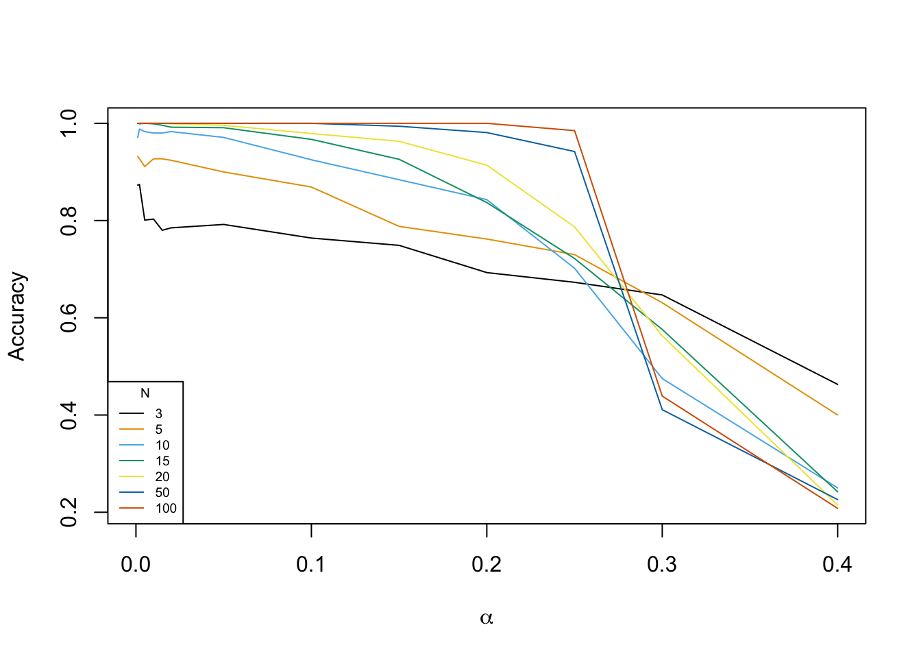
Graphically we can, obviously, see that the algorithm is the most accurate for large values of \(N\) and small values of \(\alpha\). An astonishing result, however, is the fact that for \(\alpha \geq 0.3\) the SeqEM algorithm is inversely more efficient for smaller values of \(N\) than for large values of \(N\).

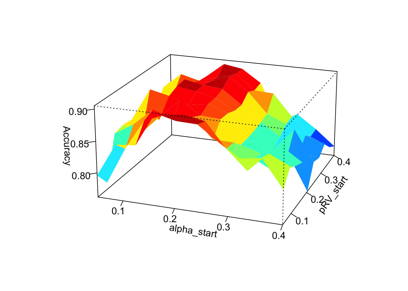
In a second experiment we want to try to conclude on the influence of the choice of the starting values of the parameters in the SeqEM algorithm. For this reason we choose to vary the starting values of 2 of the 3 parameters at the same time (thus 3 cases in total) and to observe the variation in terms of the performance of the algorithm.


S = 1000
pVV = 0.3
pRV = 0.2
alpha = 0.2
N = 15

alpha_start_values = seq(0.05,0.4,length.out=10)
pVV_start_values = seq(0.05,0.4,length.out=10)
pRV_start_values = seq(0.05,0.4,length.out=10)


# Variation of alpha_start and pVV_start
accuracies = c()
set.seed(1)
for (alpha_start in alpha_start_values){
	for (pVV_start in pVV_start_values){
	# Data simulation
	data = data_generation(S, pVV, pRV, N, alpha, getData=TRUE)
	
	# Implementation of the SeqEM algorithm
	SeqEM_result = SeqEM(data$X, alpha_start, pVV_start, pRV_start=0.1, N)
	accuracies = c(accuracies,EM_accuracy(data$Z, SeqEM_result$Z))
	}
}
accuracy_matrix_alpha_pVV = matrix(accuracies,
							nrow=length(alpha_start_values),
							ncol=length(pVV_start_values),
							byrow=TRUE,
							dimnames = list(alpha_start_values, pVV_start_values))

persp3D(alpha_start_values,pVV_start_values,accuracy_matrix_alpha_pVV,
		theta=20, phi=20, expand=0.5,
		xlab="alpha_start", ylab="pVV_start", zlab="Accuracy")


# Variation of alpha_start and pRV_start
accuracies = c()
set.seed(1)
for (alpha_start in alpha_start_values){
	for (pRV_start in pRV_start_values){
	# Simulation de données
	data = data_generation(S, pVV, pRV, N, alpha, getData=TRUE)
	
	# Implementation of the SeqEM algorithm
	SeqEM_result = SeqEM(data$X, alpha_start, pRV_start=0.1, pRV_start, N)
	accuracies = c(accuracies,EM_accuracy(data$Z, SeqEM_result$Z))
	}
}
accuracy_matrix_alpha_pRV = matrix(accuracies,
							nrow=length(alpha_start_values),
							ncol=length(pRV_start_values),
							byrow=TRUE,
							dimnames = list(alpha_start_values, pRV_start_values))

persp3D(alpha_start_values,pRV_start_values,accuracy_matrix_alpha_pRV,
		theta=20, phi=20, expand=0.5,
		xlab="alpha_start", ylab="pRV_start", zlab="Accuracy")


# Variation of pVV_start and pRV_start
accuracies = c()
set.seed(1)
for (pVV_start in pVV_start_values){
	for (pRV_start in pRV_start_values){
	# Simulation de données
	data = data_generation(S, pVV, pRV, N, alpha, getData=TRUE)
	
	# Implementation dof the SeqEM algorithm
	SeqEM_result = SeqEM(data$X, alpha_start=0.1, pVV_start, pRV_start, N)
	accuracies = c(accuracies,EM_accuracy(data$Z, SeqEM_result$Z))
	}
}
accuracy_matrix_pVV_pRV = matrix(accuracies,
									nrow=length(pVV_start_values),
							ncol=length(pRV_start_values),
							byrow=TRUE,
							dimnames = list(pVV_start_values, pRV_start_values))

persp3D(pVV_start_values,pRV_start_values,accuracy_matrix_pVV_pRV,
		theta=20, phi=20, expand=0.5,
		xlab="pVV_start", ylab="pRV_start", zlab="Accuracy")

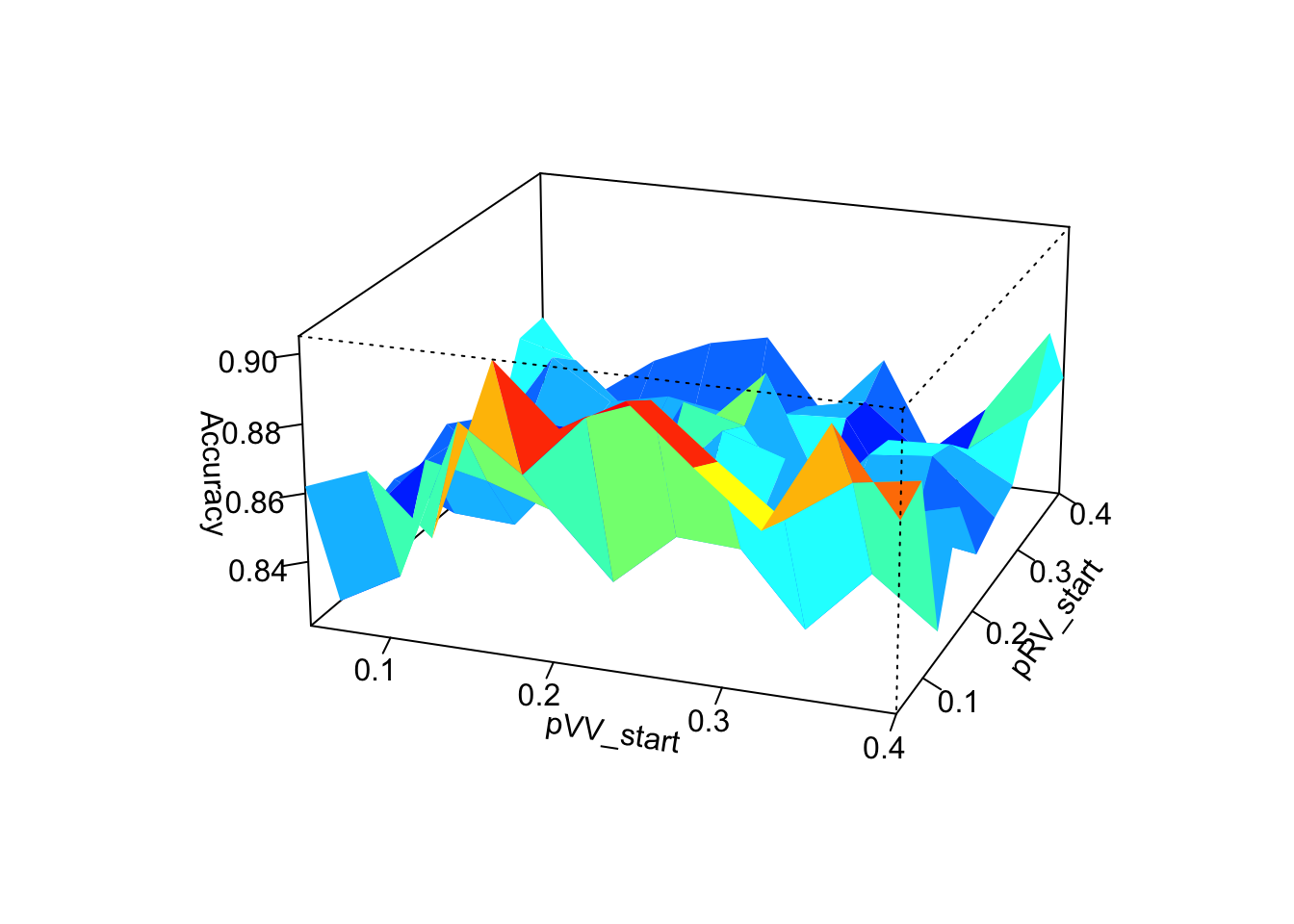
Graphically, we can clearly see that the choice of the starting value of \(\alpha\) has the greatest influence on the performance of the algorithms. The closer the chosen starting value of \(\alpha\) is to the true value of \(\alpha\) the more accurate the algorithm determines the genotypes. The choice of starting values for \(p_\text{pVV}\) and \(p_\text{RV}\) have much less influence on performance and we are not really able to identify a clear link between the choice of starting values for \(p_\text{VV}\) and \(p_\text{RV}\) and the performance of the SeqEM algorithm.

Conclusions (review + perspectives)

The idea behind the SeqEM algorithm may indeed be an interesting basis for the development of new genotyping methods or technologies. Its ease of implementation and good comprehensibility are, without doubt, desirable characteristics. On the other hand, it is rather only an introduction to these new methods, because the SeqEM algorithm has some weaknesses that must necessarily be corrected and because the assumptions for the implementation of the algorithm have been extremely simplified in the article. For example, the hypothesis of independence between individuals, which was very useful in formulating \(Q(\theta|\theta_{old})\), cannot always be satisfied. Since individuals can, for example, be related, one must be very careful when selecting individuals. Another weakness is the importance of the choice of the starting value of \(\alpha\), which was shown in the last experiment. Another factor, on which the performance of the SeqEM algorithm is highly dependent, is the read depth \(N\) and the true value of \(\alpha\). If \(N\) is large enough and \(\alpha\) is small enough, the algorithm is able to determine genotypes with high accuracy. On the other hand, for small values of \(N\) and large values of \(\alpha\) the algorithm has difficulties to properly call the true genotype. These results lead us to the conclusion that, if we manage to simplify all the hypotheses (which can certainly be difficult in reality), the SeqEM algorithm is a very interesting and easy to apply approach for genotyping. Even if the algorithm has some shortcomings, these are certainly not impossible to solve in the future, so that the SeqEM algorithm may gain popularity.

Annexe

\[\begin{equation*} \begin{cases} \displaystyle \frac{\partial Q(\theta | \theta^{\text{old}})}{\partial \alpha} = 0 \\\\ \displaystyle \frac{\partial Q(\theta | \theta^{\text{old}})}{\partial p_\text{VV}} = 0 \\\\ \displaystyle \frac{\partial Q(\theta | \theta^{\text{old}})}{\partial p_\text{RV}} = 0 \end{cases} \end{equation*}\]

\[\begin{equation*} \iff \begin{cases} \displaystyle \sum_{i=1}^{S}\left\{ \eta_{\text{VV}}(i) \left[ X_i \frac{-1}{1-\alpha} + (N_i-X_i)\frac{1}{\alpha} \right] + \eta_{\text{RR}}(i)\left[ X_i \frac{1}{\alpha} - (N_i-X_i)\frac{1}{1-\alpha} \right] \right\} = 0 \\\\ \sum_{i=1}^{S}\left\{ \eta_{\text{VV}}(i) \frac{1}{p_\text{VV}} - \eta_{\text{RR}}(i) \frac{1}{1-p_\text{VV}-p_\text{RV}} \right\} = 0 \\\\ \sum_{i=1}^{S}\left\{ \eta_{\text{RV}}(i) \frac{1}{p_\text{RV}} - \eta_{\text{RR}}(i) \frac{1}{1-p_\text{VV}-p_\text{RV}} \right\} = 0 \end{cases} \end{equation*}\]

Since the first equation depends only on \(\alpha\) and the other two equations depend only on \(p_\text{VV}\) and \(p_\text{RV}\), the system of equations can be divided into 2 parts. We start by solving the first equation:

\[\begin{align*} & \sum_{i=1}^{S}\left\{ \eta_{\text{VV}}(i) \left[ X_i \frac{-1}{1-\alpha} + (N_i-X_i)\frac{1}{\alpha} \right] + \eta_{\text{RR}}(i)\left[ X_i \frac{1}{\alpha} - (N_i-X_i)\frac{1}{1-\alpha} \right] \right\} = 0 \\ \iff & \sum_{i=1}^{S}\left\{ \eta_{\text{VV}}(i) \left[ -\alpha X_i + (1-\alpha)(N_i-X_i) \right] + \eta_{\text{RR}}(i)\left[(1-\alpha) X_i - \alpha (N_i-X_i) \right] \right\} = 0 \\ \iff & \sum_{i=1}^{S}\left\{ \eta_{\text{VV}}(i) \left[ N_i - \alpha N_i - X_i \right] + \eta_{\text{RR}}(i)\left[X_i - \alpha N_i \right] \right\} = 0 \\ \iff & \alpha \sum_{i=1}^{S}\left\{ \eta_\text{VV}(i) N_i + \eta_\text{RR}(i) N_i \right\} = \sum_{i=1}^{S} \left\{ \eta_{\text{VV}}(i) \left[ N_i - X_i \right] + \eta_{\text{RR}}(i) X_i \right\} \\ \iff & \boxed{\alpha_{new} = \frac{\displaystyle \sum_{i=1}^{S} \left\{ \eta_{\text{VV}}(i) \left[ N_i - X_i \right] + \eta_{ \text{RR}}(i) X_i \right\}}{\displaystyle \sum_{i=1}^{S}\left\{N_i \left[\eta_\text{VV}(i) + \eta_\text{RR}(i) \right] \right\}}} \end{align*}\]

We continue by solving the system of equations composed of the two other equations of the initial system.

\[\begin{align} &\begin{cases} \sum_{i=1}^{S}\left\{ \eta_{\text{VV}}(i) \frac{1}{p_\text{VV}} - \eta_{\text{RR}}(i) \frac{1}{1-p_\text{VV}-p_\text{RV}} \right\} = 0 \\\\ \sum_{i=1}^{S}\left\{ \eta_{\text{RV}}(i) \frac{1}{p_\text{RV}} - \eta_{\text{RR}}(i) \frac{1}{1-p_\text{VV}-p_\text{RV}} \right\} = 0 \end{cases} \nonumber \\ \iff &\begin{cases} \sum_{i=1}^{S}\left\{ \eta_{\text{VV}}(i) \frac{1}{p_\text{VV}} \right\} = \sum_{i=1}^{S}\left\{ \eta_{\text{RR}}(i) \frac{1}{1-p_\text{VV}-p_\text{RV}} \right\} \\\\ \sum_{i=1}^{S}\left\{ \eta_{\text{RV}}(i) \frac{1}{p_\text{RV}} \right\} = \sum_{i=1}^{S}\left\{ \eta_{\text{RR}}(i) \frac{1}{1-p_\text{VV}-p_\text{RV}} \right\} \end{cases} \label{eq1} \end{align}\]

\[\begin{align} \Longrightarrow & \sum_{i=1}^{S}\left\{ \eta_{\text{VV}}(i) \frac{1}{p_\text{VV}} \right\} = \sum_{i=1}^{S}\left\{ \eta_{\text{RV}}(i) \frac{1}{p_\text{RV}} \right\} \nonumber \\ \iff & p_\text{RV} \sum_{i=1}^{S} \eta_{\text{VV}}(i) = p_\text{VV} \sum_{i=1}^{S} \eta_{\text{RV}}(i) \nonumber \\ \iff & p_\text{RV} = p_\text{VV} \frac{\sum_{i=1}^{S} \eta_{\text{RV}}(i)}{ \sum_{i=1}^{S} \eta_{\text{VV}}(i)} \label{eq2} \end{align}\]

Using this equality in the first system of equations (1), we find that

\[\begin{align*} & \left[ \sum_{i=1}^{S} \eta_{\text{VV}}(i) \right] \times \frac{1}{p_\text{VV}} = \left[ \sum_{i=1}^{S} \eta_{\text{RR}}(i) \right] \times \frac{1}{1-p_\text{VV}-p_\text{VV} \frac{\sum_{i=1}^{S} \eta_{\text{RV}}(i)}{ \sum_{i=1}^{S} \eta_{\text{VV}}(i)}} \\ \iff & \left[ \sum_{i=1}^{S} \eta_{\text{VV}}(i) \right] \times \left[ 1-p_\text{VV}-p_\text{VV} \frac{\sum_{i=1}^{S} \eta_{\text{RV}}(i)}{ \sum_{i=1}^{S} \eta_{\text{VV}}(i)} \right] = \left[ \sum_{i=1}^{S} \eta_{\text{RR}}(i) \right] \times p_\text{VV} \\ \iff & p_\text{VV} \times \left[\underbrace{\sum_{i=1}^{S} \eta_{\text{RR}}(i) + \sum_{i=1}^{S} \eta_{\text{VV}}(i) + \sum_{i=1}^{S} \eta_{\text{RV}}(i)}_{S \text{ , car } \eta_{\text{VV}}(i)+\eta_{\text{RV}}(i)+\eta_{\text{RR}}(i)=1} \right] = \sum_{i=1}^{S} \eta_{\text{VV}}(i) \\ \iff & \boxed{p_\text{VV}^{new} = \frac{\displaystyle \sum_{i=1}^{S} \eta_{\text{VV}}(i)}{\displaystyle S}} \end{align*}\]

Using this result in the second system of equations (2), we find that \[\boxed{p_\text{RV}^{new} = \frac{\displaystyle \sum_{i=1}^{S} \eta_{\text{RV}}(i)}{\displaystyle S}}\]